Epilepsy 101 for Computational People

Disclaimer: This document cannot be used as any ground for medical and legal purposes. I write this up just because I am tired of explaining basic epilepsy terms to my colleagues (informatists, not neurologists) again and again.

1. Epilepsy is a neurological disorder while seizure is a characteristic symptom of epilepsy. Jerks are one kind of seizures.
2. In 1981, ILAE made a seizure classification that is widely used until today
   
   1. Focal Seizures: seizure limited in or originated from one hemisphere of the brain
      
      1. simple partial seizures, (simple: no interruption on consciousness)
      2. complex partial seizures, (complex: with interruption on consciousness) and
      3. partial seizure evolving into secondary generalized seizures, about 1/3 of partial seizures
   2. (Primary) Generalized Seizures: seizure all over the brain
      
      1. absence seizures (kinda like blackout), formerly called petit mal
      2. tonic-clonic seizures (kinda like whole-body jerk), formerly called grand mal
      3. many other generalized seizures
   3. Unclassified epileptic seizures
3. In 1989, ILAE made an epilepsy classification that is widely used until today
   
   1. Focal Epilepsies
      
      1. sympotomatic or cryptogenic (cause unknown): e.g., temporal lobe epilepsy (TLE)
      2. idopathic (genetic causes): e.g., benign childhood epilepsy
   2. Generalized Epilepsies
      
      1. sympotomatic or cryptogenic (cause unknown): e.g., West syndrome, Lennox-Gastaut syndrom
      2. idiopathic: e.g., childhood absence epilepsy, juvenile absence epilepsy,
   3. Epilepsies undertermined whether focal or generalized
4. When seizure is onset, we say the subject is in ictal state. Otherwise, interictal state. Because seizure duration (few seconds/minutes) is much shorter compared with interictal period, interictal EEG is more accessible.
5. EEG is a gold standard for epilepsy diagnosis. However, neurologists heavily rely on either ictal EEG or interictal epileptiform discharges (IEDs, such as sharp wave and spikes) in diagnosis. The IEDs are the distinctive EEG patterns for epilepsy when subjects are not in seizure. Because seizure and IEDs happen unpredictably and sporadically, the way to catch them is to use long-term EEG recordings which can last from hours to days. Such tedious procedure is costly and inconvenient.
6. Typical signal processing and machine learning problems related to epileptic EEG
   
   1. coarse epilepsy diagnosis: distinguishing epileptic interictal EEG (with or without IEDs) and non-epileptic EEG
   2. fine epilepsy/seizure diagnosis: identifying the type of seizure and/or epilepsy based on ictal or interictal EEG
   3. seizure detection: detecting seizure activities from epileptic subjects' EEG
   4. seizure prediction: predicting the onsets of seizure activities from epileptic subjects' EEG
   5. focus localization: locating the epileptogenic zone (for focal seizures only)

References:
1. For complete list of seizure types and epilepsy types, check Tables 9-1 and 9-2 on Pages 121-122 of this doc from British gov: http://www.nice.org.uk/guidance/cg137/resources/cg137-epilepsy-full-guideline3 which are reprinted from 1981 and 1989 ILAE classifications.

Reading Physiology Data in EDF+ Format Using EEGTools

For years, I always converted EDF+ format data into text files for processing. Recently, I was tired of this and decided to try directly read EDF+ data. I tried out a Python module EEGTools by Boris Reuderink and it turned out to be great. It's super easy to use. Just use these two lines:

import eegtools
Data = eegtools.io.load_edf('Sample.edf')

The structure of Data is like this

EDF(X=array([[ -14.,    9.,  -70., ...,  -50.,  -99.,  -93.],
       [ -35.,  -21.,  -87., ...,  -45.,  -98.,  -81.],
       [ -72.,  -62., -116., ...,  -32.,  -79.,  -52.],
       ..., 
       [ -37.,  -89.,  -63., ...,  -41.,  -16.,  -45.],
       [ -69., -120.,  -99., ...,  -46.,  -25.,  -55.],
       [ -44.,  -87.,  -57., ...,  -29.,   -4.,  -41.]], dtype=float32), sample_rate=160.0, chan_lab=['Fc5.', 'Fc3.', 'Fc1.', 'Fcz.', 'Fc2.', 'Fc4.', 'Fc6.', 'C5..', 'C3..', 'C1..', 'Cz..', 'C2..', 'C4..', 'C6..', 'Cp5.', 'Cp3.', 'Cp1.', 'Cpz.', 'Cp2.', 'Cp4.', 'Cp6.', 'Fp1.', 'Fpz.', 'Fp2.', 'Af7.', 'Af3.', 'Afz.', 'Af4.', 'Af8.', 'F7..', 'F5..', 'F3..', 'F1..', 'Fz..', 'F2..', 'F4..', 'F6..', 'F8..', 'Ft7.', 'Ft8.', 'T7..', 'T8..', 'T9..', 'T10.', 'Tp7.', 'Tp8.', 'P7..', 'P5..', 'P3..', 'P1..', 'Pz..', 'P2..', 'P4..', 'P6..', 'P8..', 'Po7.', 'Po3.', 'Poz.', 'Po4.', 'Po8.', 'O1..', 'Oz..', 'O2..', 'Iz..'], time=array([  0.00000000e+00,   6.25000000e-03,   1.25000000e-02, ...,
         1.22981250e+02,   1.22987500e+02,   1.22993750e+02]), annotations=[(0.0, 4.1, [u'T0']), (4.1, 4.1, [u'T1']), (8.2, 4.1, [u'T0']), (12.3, 4.1, [u'T2']), (16.4, 4.1, [u'T0']), (20.5, 4.1, [u'T2']), (24.6, 4.1, [u'T0']), (28.7, 4.1, [u'T1']), (32.8, 4.1, [u'T0']), (36.9, 4.1, [u'T2']), (41.0, 4.1, [u'T0']), (45.1, 4.1, [u'T1']), (49.2, 4.1, [u'T0']), (53.3, 4.1, [u'T2']), (57.4, 4.1, [u'T0']), (61.5, 4.1, [u'T1']), (65.6, 4.1, [u'T0']), (69.7, 4.1, [u'T1']), (73.8, 4.1, [u'T0']), (77.9, 4.1, [u'T2']), (82.0, 4.1, [u'T0']), (86.1, 4.1, [u'T1']), (90.2, 4.1, [u'T0']), (94.3, 4.1, [u'T2']), (98.4, 4.1, [u'T0']), (102.5, 4.1, [u'T1']), (106.6, 4.1, [u'T0']), (110.7, 4.1, [u'T2']), (114.8, 4.1, [u'T0']), (118.9, 4.1, [u'T1'])])

As you can see, the recordings are in the member X. The channels that member arrays of X correspond to are sequentially given in the member chan_lab. Sampling rate and time instants are given in sample_rate and time. Lastly, you can access the annotation on EEG from annotations.

To download or install, see EEGTools' GitHub page: http://borisreuderink.nl/ Read the instruction at the bottom and use PIP to install - easier than cloning and setup.py.

The schematic for my ECG sampling circuit

by Forrest Sheng Bao http://fsbao.net

So here is the schematic of my ECG sampling circuit. I designed the circuit in fall 2010.

I would like to say that TI's(well, Burr-Brown's) instrumentation amplifier is awesome. You just put things together and then they rock. No need to tune the peripheral circuit. It's kinda like out-of-the-box solutions. Since the gain can be very high (10000 times linear), i think they can even be used for EEG sampling circuit.

I did not build the ADC circuit and interface to computers, but used NI myDAQ. The power supply for this circuit is also provided by NI myDAQ.

There are three electrodes connected to human body, the belly (ground), the left wrist (one input), and the right wrist (the other input).

This circuit can also sample signals output from NI myDAQ back to test the property of the circuit. Since the lowest resolution to NI myDAQ is 100mV, i used an op-amp (OPA177) as a voltage divider to scale down the output signal from NI myDAQ to its 1/10 (in voltage amplitude).

The schematic was drawn by gEDA/gschem. Click to enlarge.

high resolution ADC vs. high-gain amplifier: A lesson from Bode Analyzer of NI myDAQ

by Forrest Sheng Bao http://fsbao.net

Around a month ago, I met an engineer from an EEG sampling system company. I asked him many specifications of their circuit. He told me that they only amplify the EEG signal by 20 or 30 times and then feed it to a 24-bit ADC. Besides noise issues,  did not understand why they chose high-resolution ADC over high-gain amplifier. Today I learned a lesson and figured out.

I am using NI myDAQ these days to test the amplification (very high gain, expected to be 10,000 or 80dB) circuit I prepared for ECG data acquisition project. Of course, Bode plot is what I used to the check the gain and phase shift.

My configuration. The chip on the left is an TI OPA177 used to divide the input voltage of INA128 to as low as 1mV. The minimum resolution of the Function Generator of NI myDAQ is 10mV and I wanted the signal amplitude to be as low as raw ECG. The chip on the right is TI INA128, with R_G set as 5 Ohm. The output signal of INA128 is filtered by an RC bandpass filter and then goes to myDAQ. There was an error in the circuit when I shot this picture. The ground of RC circuit was not grounded.

Any analog circuit has a setting time (at least the speed of light), e.g., to reach a feedback balance. When the gain of an amplifier goes very high, the setting time increases nonlinearly. According to the datasheet (http://www.ti.com/lit/gpn/ina128) from Texas Instruments, the setting time of instrumentation amplifier INA128 is 9 us when gain is 100 while 80 us when gain is 1000. The gain of INA128 ranges from 1 to 10000. But the datasheet does not say what will happen for gain larger than 1000. Why? Probably because the setting time is very long and varies from device to device.

This is like many bivariate constraints in analog circuit design, e.g., gain-bandwidth product. Therefore, in Bode analysis, it needs to wait significant long enough time before you can measure the output and move the next frequency. 

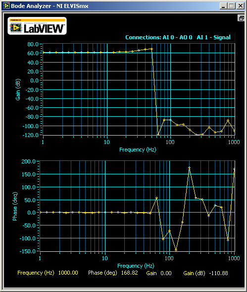
But the Bode Analyzer that comes with NI myDAQ (also used on NI ElVIS II/II+), does not give the circuit enough setting time. The software measures the output before the circuit can settle down from the input stimulus.

What happened was, when gain is 1000, I saw this

I said, what? Where are my signals over 14 Hz? But when I increase the gain to 5000 (well, from myDAQ's oscilloscope which now I assume has errors too because the theoretical gain for my configuration is 10,000.), I was thinking to withdraw this class:

The gain was constantly high before 10 Hz and dropped drastically after that. The phase shifting plot looked like stock market after that. According to the datasheet of INA128, the gain should not drop before 1kHz.

Why? Now I know the answer, because the Bode Analyzer did not wait until the circuit to stabilize. It measured unstable output. As the gain goes higher, more waiting time is needed.

But at that moment, I did not think about this. I tried another way to study the problem, using other instruments. I checked the waveform on the Oscilloscope of NI myDAQ while letting the Function Generator of myDAQ sweep from 1 Hz to 20Hz, with a step of 0.5 Hz. And, I let the signal stay at each frequency for 3 second, way enough for the circuit to stabilize. By comparing the Vp-p on the oscilloscope, I saw that my circuit wasn't as bad as the Bode plot showed. It was as designed.

Below is a video I took when the Function Generator swept. I didn't save the original video for the output from INA128. Instead, I recorded the output waveform from an RC bandpass filter following the output of INA128 (blue line). The green line was the input to INA128. I set the cutoff frequency of the RC filter at 15Hz (which is not exact because the discrete components have 5% error each). As you can see, the signal drops gradually after 8Hz but not at a >100dB attenuation. Also, the phase shift wasn't as crazy as stock market. The shift was almost invisible. Of course, I need to fix the circuit because apparently, the -3-dB point was at 22Hz (not shown on the screen as I ended the screencast early).



So, go back to my question, why medical instruments prefer high-resolution ADC over high-gain amplifier, besides noise issues. Well, a high-gain amplifier takes long time to stabilize (INA128 takes 80us to set at G=1000), then the sampling rate cannot be high (for INA128, sampling rate can not be higher than 10kHz when G=1000). The setting time for amplifiers at high gain, is longer than the setting time of a high-resolution ADC (which can handle MHz signal).

PS: Another interesting thing is that Bode Analyzer of myDAQ gave me this for TI INA101:

 I would like to know whether INA101 is really bad from 1 to 10 Hz or it's another problem of the Bode Analyzer of myDAQ.

Do computers know EEG reading?

This is how neurologists check frequencies and amplitudes of EEG signals in the old days - I found this card from the back cover of a Japanese book (2006) about EEG reading.

The method is matching boxes, e.g., 1-30, to EEG waves. If the number of peaks matches box n, then the frequency of the wave is n Hz. Of course, a wave can have many frequency components and thus matches several boxes on different amplitudes, like lower frequencies modulated onto higher frequencies - just imaging how sin(x)*sin(4x) look like in your high school math class.

Now, with computerized EEG recordings, neurologists still are using this way to diagnose. The only difference is that the boxes on the card are replaced by different background rulers on computer screens. So are amplitude rulers.

The question is, whether representing the knowledge and methods from physicians is the only way we can teach computers to read EEG? If this is the only possible track, then how we can teach computers to identify different wave patterns, in time domain?  If the answer is yes, then a lotta work done in these years about spike detection is a killer approach.

But, "do submarines swim?" "They just don't swim in the way you swim." Dr. Dijkstra, who served as Computer Science Department chair at UT Austin between 1984- 2000.

So, another approach is to teach computers a whole new way to mathematically analyze EEG waveforms, not following the way that physicians use which identifies particular EEG patterns, like spike-slow waves. For example, we may teach computers that the skews in this EEG is different from skews in another EEG.

EEG Signal Processing in Python and Scipy.Signal (1): Spectrum Estimation, FIR Filter Design, Convolution and Windowing

by Forrest Sheng Bao http://fsbao.net

(Update 2012-12-22: People have been asking about the input format of the EEG data. Well, there is no input - because I didn't use any function. My code loads data from a text file (a TSV one), where rows correspond to sampling instant sequentially and columns correspond to channels. Therefore, you just need to ensure that the variable eeg is a 2-D list or numpy array such that any row is sublist/subarray representing the value from all channels at a sampling time. For example, if you have only two sampling instants for a 4-channel EEG, you would expect eeg to be like [[1,2,3,4],[5,6,7,8]].)

I am doing a take-home midterm test of a class I am taking. So, I decided to use Python to to it. Below is a code for one problem. It includes several frequency used functions in classical signal spectral analysis and FIR filter design. The problem itself is to design bandpass filters over alpha to theta bands and apply them onto a EEG series, and plot the time domain and frequency domain signal, as well as the frequency response of filters. I used window methods to design FIR bandpass filters. The filters coefficients are smoothed by a Kaiser window. Filtering is implemented by convolving original signal with coefficients of filters.

The result of running this code is given below. Black lines in the bottom plot is the amplitude property of different filters. As you can see, signals outside filter bands are kicked out respectively.

# This software is a free software that comes with NO WARRANTY
# You have the right to obtain, modify and redistribute this code 
# under the terms of  GNU General Public License ver. 3 or later
# Copyleft 2009 Forrest Sheng Bao http://fsbao.net

from numpy import *
from scipy.signal import *
from numpy.fft import * 
from matplotlib import *
from scipy import *
from pylab import *

f=open('./EEG1_1c31.txt','r')
chno = 16   # total number of channels
eeg = [] 

while True:
 testline = f.readline()
 if len(testline) == 0:
  break #EOF
 testline = testline.split()
 eeg.append([])
 for i in xrange(0,chno):
  eeg[-1].append(float(testline[i])) 

ch = 1 # particualr channel to study 
eeg = array(eeg)
y = eeg[:,ch]         # the signal, study channel 'ch'
L = len(y)            # signal length
fs = 500.0              # sampling rate
T = 1/fs                # sample time
t= linspace(1,L,L)*T   # time vector

f = fs*linspace(0,L/10,L/10)/L  # single side frequency vector, real frequency up to fs/2
Y = fft(y)

figure()
filtered = []
b= [] # store filter coefficient
cutoff = [0.5,4.0,7.0,12.0,30.0]

for band in xrange(0, len(cutoff)-1):
 wl = 2*cutoff[band]/fs*pi
 wh = 2*cutoff[band+1]/fs*pi
 M = 512      # Set number of weights as 128
 bn = zeros(M)
 
 for i in xrange(0,M):     # Generate bandpass weighting function
  n = i-  M/2       # Make symmetrical
  if n == 0:
   bn[i] = wh/pi - wl/pi;
  else:
   bn[i] = (sin(wh*n))/(pi*n) - (sin(wl*n))/(pi*n)   # Filter impulse response
 
 bn = bn*kaiser(M,5.2)  # apply Kaiser window, alpha= 5.2
 b.append(bn)
 
 [w,h]=freqz(bn,1)
 filtered.append(convolve(bn, y)) # filter the signal by convolving the signal with filter coefficients

figure(figsize=[16, 10])
subplot(2, 1, 1)
plot(y)
for i in xrange(0, len(filtered)):
  y_p = filtered[i]
  plot(y_p[ M/2:L+M/2])
axis('tight')
title('Time domain')
xlabel('Time (seconds)')

subplot(2, 1, 2)
plot(f,2*abs(Y[0:L/10]))
for i in xrange(0, len(filtered)):
  Y = filtered[i]
  Y = fft(Y [ M/2:L+M/2])
  plot(f,abs(Y[0:L/10]))
axis('tight')
legend(['original','delta band, 0-4 Hz','theta band, 4-7 Hz','alpha band, 7-12 Hz','beta band, 12-30 Hz'])

for i in xrange(0, len(filtered)):   # plot filter's frequency response
  H = abs(fft(b[i], L))
  H = H*1.2*(max(Y)/max(H))
  plot(f, 3*H[0:L/10], 'k')    
axis('tight')
title('Frequency domain')
xlabel('Frequency (Hz)')
subplots_adjust(left=0.04, bottom=0.04, right=0.99, top=0.97)
savefig('filtered.png')

Reference: Signal Processing Toolbox of Scipy, http://docs.scipy.org/doc/scipy/reference/signal.html

EDFbrowser working with discontinuous EDF+ file

by Forrest Sheng Bao http://fsbao.net

EDFbrowser is an open source EDF Browser. EDF/EDF+ is an open file format for biomedical time series, especially EEG and ECG/EKG signal.

But, the pain is, new (version 1.08 or later) EDFbrowswer "disabled the possibility to open discontinuous files."

I consulted the author, Teunis van Beelen, and got a solution from him.

1. Open the file mainwindow.cpp in a texteditor.
2. Comment the lines 1293 to 1310. Put /* and */ at the beginning and end of following code

   if(edfhdr->discontinuous)
   {
   if(edfhdr->edf)
   {
     UI_Messagewindow popuperror("Error", "EDFbrowser can not show EDF+D (discontinuous) files.\n"
                                 "Convert this file to EDF+C first. You can find this converter\n"
                                 "in the Tools menu (EDF+D to EDF+C converter).");
   }
   
   if(edfhdr->bdf)
   {
     UI_Messagewindow popuperror("Error", "EDFbrowser can not show BDF+D (discontinuous) files.\n"
                                 "Convert this file to BDF+C first. You can find this converter\n"
                                 "in the Tools menu (EDF+D to EDF+C converter).");
   }
   
   free(edfhdr->edfparam);
   free(edfhdr);
   fclose(newfile);
   
   return;
   }

   Now compile the source code by executing qmake && make and you are done.

Modifying this source code and recompiling it is legal since this software is distributed under GNU GPL v 2.

Time stamp issues in EDF data converted from Stellate SIG format

by Forrest Sheng Bao http://fsbao.net

I think there is obvious a bug in Stellate Hamonie system, the software to sample data from EEG electrodes and manage them, convert them into EDF format. Actually, the EDF data converted from SIG has many problems, time stamps in wrong order, time stamps of wrong seconds, all-zero amplitudes, incorrect starting time, etc. I spent a lot of time to understand what's going on. At first, I was even frustrated that I couldn't use those data. Let's have a look at the data of their own SIG format and the data of EDF file converted from it.

This is the snapshot of viewing one channel data from their software, the Hamonie. The resolution of Y-axe is 10uV/mm while the time interval between two vertical green bars is 1 second.

This is the plot from EDF file converted by Hamonie, of the same data as above picture. The Y ticks are voltages in uV while the X ticks are numbers of sampling points (200 points = 1 second).

At first, the sign of above two images are opposite. This is because by default, the polarity in Stellate Hamonie system is negative up. Thus, their Y-axes is up-side-down. You can't change this setting in version 6.1, the one I got from the Chinese hospital. In version 6.2 of Stellate Browser, you can set it. Just click menu "Channels" -> "Edit", and set "Polarity" by clicking "Pos. Up" as follows:

The time stamps in EDF data have more problems. I used the Amplitude-Time cursor tool (In Stellate Browser menu: Tools -> Amplitude-Time curcor) to check exactly the value of each points on SIG data, and compare with those in EDF format data.

1. The time stamp of the first sampling point.

Firstly, according to EDF+ protocol, the time stamp of the first sampling point should be 0, which means the starting time of the series. If you sampling rate is 200Hz, then the time stamp of the second point is 0.005 - 0.005 second after the start. That makes the data I got can't pass the EDF compatibility test in several software. Let's have a look at the first sampling point of the EDF file:

23.303000,7.782218,-15.717028,5.035553,-9.765921,3.814813,-2.136295,4.272590,7.171848,9.765921,13.580733,19.837026,-30.060724,10.681476,-1.831110,-4.882960,11.749623,7.477033,-8.392588,13.580733,1.678518,-2.746665,11.597031

The 23.303 means this point is sampled 23.303 second after the record starts. Entries delimited by commas corresponds to signals defined in EDF header. For example, the 7.782218 corresponds to the Fp1 electrode.

I felt very confused about the relationship between the time stamps and time instants in SIG file. So I did a small experiment. I tried to read amplitude of first several samples of SIG data from Stellate Browser, and compared them with data read from EDF file.

	Time stamp on SIG data	Time stamp on EDF data	Amplitude on SIG data (uV)	Amplitude on EDF data (uV)
Sample #1	17:22:51:305	23.303	8	7.782128
Sample #2	17:22:51:310	23.308	19	18.768878
Sample #3	17:22:51:315	23.313	8	8.239995
Sample #4	17:22:51:320	23.318	12	12.20741
Sample #5	17:22:51:325	23.323	6	4.425183

Ok, so I think i don't need to care the time stamp. Each line follows the order.

2. Time stamps for any arbitrary interval

The doctors in China will tell me the time of ictal activities in form of absolute clock, like 22:23:34 Jun.03, 2008. I need to be able to locate the sampling point corresponding to a give time instant.

I did another verification to make sure the relationship is linear. As you can see from above two snapshots, there is a big peak, whose amplitude excesses 100uV, at round 5.5 second, thus the 1100th sample. Here are the data for that area:

	Time stamp on SIG data	Time stamp on EDF data	Amplitude on SIG data (uV)	Amplitude on EDF data (uV)
Sample #1109	17:22:56:850	28.842	109	108.951051
Sample #1110	17:22:56:855	28.847	109	109.408828
Sample #1111	17:22:56:860	28.852	92	92.103282
Sample #1112	17:22:57:865	28.857	78	78.432549
Sample #1113	17:22:57:870	28.852	76	76.143661
Sample #1114	17:22:57:875	28.862	84	83.925879
Sample #1115	17:22:57:880	28.867	112	112.308086
Sample #1116	17:22:57:885	28.872	98	97.506612
Sample #1117	17:22:57:890	28.877	80	79.500697
Sample #1118	17:22:57:895	28.882	85	85.146619
Sample #1119	17:22:57:900	28.887	104	104.373275

I think my guessing is correct. The time between the 1st and the 1100th sampling is (1110-1) x 0.005 = 5.545 seconds. The time stamp of sample 1110 in SIG data should be 17:22:51.305 + 5.545s = 17.22.56.850. The time stamp of sample 1110 in EDF data should be 23.303 + 5.545 = 28.848. It's not 28.847! I checked the data and found the problem. The time stamp of the 200th sample is 24.298 while the one of the 201th sample is 24.302. I am not quite sure about the reason. Anyway, it's not a big deal.

3. Time stamps of last 1 second

The time stamp of the last 1 second is totally nonsense. The time stamp can jump from 36.297 to 0. In the data above, from 2601st sample to 2687th sample, the time stamps are from 0 to 0.430. The last time stamp of SIG data is 17:23:04.735, which should correspond to the 2687th sample ((17:23:04.735 - 17:22:51.305) x 200 +1 = 2687). But, the EDF file has the 2688th sample. What's wrong? Let's have a look at the samples 2685 to 2688:

	Time stamp on SIG data	Time stamp on EDF data	Amplitude on SIG data (uV)	Amplitude on EDF data (uV)
Sample #2685	17:23:04:720	0.420	-21	-21.363
Sample #2686	17:23:04:725	0.425	-12	-12.0548
Sample #2687	17:23:04:730	0.430	-15	-14.8015
Sample #2688	There is no such sample in SIG data	0.435	There is no such sample in SIG data	-14.3437

So I still don't know where does the 2688th sample come from. Just neglect it.

4. All 0's record

From 0.44 second to 0.995 second in EDF data, amplitudes of all channels are zero's. I think maybe the Stellate Hamonie system wanna pad one complete second. Anyway, those data, just forget them.

5. The time the record starts

As i said before, I need the starting time of a record to determine the number of samples to a given arbitrary absolute time. This is also funny. On the SIG data, it says the record starts from 17:22:51.305. But in the EDF head, it says: 17:22:28. I checked the header information of SIG data, it is also 17:22:28. So what happened from 17:22:29 to 17:22:23?

Anyway, this is not a problem since I have figured out the relationship between time stamps in SIG data and EDF data. I just need to consider the time stamp of first sample in SIG data as the starting time.

Done!

Ok, so it is really hard to understand a format that you don't know before, along with that strange software. I still have some problem, the actual data of long-term EEG monitoring is very big, like 2G or 3G. But my old program load the entire data into the computer memory. Now, it is impossible. I need to play some programming tricks.

Converting Stellate SIG format EEG data into EDF and ASCII

by Forrest Sheng Bao http://fsbao.net

Stellate is a company developing EEG sampling and analysis system in Montreal, Canada. Their system is good. But unlike many other software developed in Montreal Neurological Institute, McGill U., it runs on Windows! So, I tried to install it on Linux thru wine, another open source project aiming to run Windows application on Linux. Cool, it is very easy. Just 2 minutes work. Here displays a short segment of 7 seconds in resolution 7.5 uV/mm. The format, SIG, Stellate system uses is a proprietary format. Thus, we can't apply any our own algorithms onto the data sampled in their system. They provided one way to export the data into EDF (European Data Format) files. Then I can open them by another open source software, EDF Browser, developed by Teuniz, a guy in Leiden University, Netherlands. This is the snapshot of EDFBrowser. The data are the same as above snapshot. But, I found a funny problem: They have opposite signs. So the data are upside down. There is also a bug in the EDF file exported from Stellate system. Let's look at the EDF records of above plot. It starts like this:

Time,1,2,3,4,5,6,7,8,9,10,11,12,13,14,15,16,17,18,19,20,21,22
23.303000,7.782218,-15.717028,5.035553,-9.765921,3.814813,-2.136295,4.272590,7.171848,9.765921,13.580733,19.837026,-30.060724,10.681476,-1.831110,-4.882960,11.749623,7.477033,-8.392588,13.580733,1.678518,-2.746665,11.597031
23.308000,18.768878,-5.035553,14.801473,1.525925,13.733326,8.545180,13.428141,19.074063,16.022213,26.551096,28.992576,-16.327398,17.395546,10.376291,3.967405,22.278506,18.005916,4.425183,14.343696,11.902216,5.798515,23.957024
23.313000,8.239995,-16.785176,7.477033,-5.188145,8.239995,1.678518,8.545180,12.054808,13.428141,19.074063,18.311101,-25.482949,8.087403,-0.915555,-4.119998,12.207401,8.087403,-8.850365,9.918513,6.561478,0.610370,17.853323
23.318000,12.207401,-13.428141,11.902216,-1.983703,14.496288,3.509628,14.038511,12.817771,19.989619,19.837026,19.531841,-25.025171,14.801473,0.762963,1.220740,13.580733,7.934810,-7.477033,13.428141,11.139253,5.951108,19.684434
23.323000,4.425183,-17.090361,5.493330,-12.054808,8.087403,-5.798515,8.697773,3.357035,15.106658,11.444438,14.801473,-32.502204,3.357035,-6.561478,-5.188145,2.746665,4.119998,-15.106658,9.308143,4.882960,-0.305185,11.444438
23.328000,12.207401,-11.291846,13.122956,-6.103700,14.648881,1.220740,14.343696,9.765921,21.668136,15.717028,21.210359,-25.330356,11.749623,0.457778,1.831110,5.645923,9.460735,-11.902216,19.074063,12.359993,7.324440,17.700731
23.333000,7.782218,-23.346654,4.272590,-12.359993,3.662220,-4.577775,3.357035,3.509628,13.428141,7.171848,15.869621,-31.434057,2.441480,-8.239995,-4.882960,-1.220740,3.204443,-18.311101,10.376291,5.340738,0.305185,11.291846
23.338000,14.954066,-13.733326,10.376291,-2.746665,10.681476,5.188145,9.613328,11.902216,21.820729,15.106658,24.414801,-23.041469,8.545180,-3.967405,1.373333,3.204443,12.665178,-8.392588,14.496288,13.122956,7.782218,17.548138
23.343000,5.798515,-19.837026,1.831110,-9.460735,2.288888,-1.831110,0.305185,2.746665,12.054808,6.866663,14.801473,-31.434057,4.272590,-18.005916,-6.714070,-3.967405,2.594073,-16.022213,6.866663,5.035553,1.220740,10.223698

Since the sampling rate is 200 Hz, the difference between two consecutive timestamps is 5 ms. The first field of each line represents the time after the exam begins. It is followed by voltages of all channels. For example, the voltage of first channel at 23.303s of the exam is 7.782218 uV. Duration of this record is from 23.303s to 30.297s. But I can find such records after that

0.000000,-5.340738,-4.425183,-0.915555,7.171848,-4.882960,2.288888,-0.152593,2.441480,-4.119998,-5.798515,-32.959982,9.308143,-12.970363,-5.035553,3.357035,-10.834068,-21.210359,-6.103700,-15.259251,-1.220740,-0.152593,-1.068148
0.005000,-8.545180,1.678518,-5.493330,-4.577775,-10.986661,-4.577775,-6.256293,-3.662220,-9.765921,-12.359993,-33.265167,3.051850,-14.496288,-3.967405,-3.967405,-17.548138,-18.921471,-11.291846,-19.379248,-7.477033,-6.561478,-7.019255
0.010000,-2.136295,5.493330,0.152593,3.662220,-3.967405,3.204443,0.000000,4.577775,-2.746665,0.152593,-25.025171,2.136295,-8.545180,-4.730368,2.288888,-9.460735,-16.785176,-6.103700,-5.035553,-0.610370,-0.610370,0.305185
0.015000,-6.103700,2.288888,-7.629625,-3.967405,-12.207401,-6.408885,-9.613328,-6.561478,-13.428141,-15.106658,-31.891834,1.831110,-12.207401,-5.188145,-6.866663,-19.837026,-18.921471,-10.071106,-17.853323,-10.834068,-9.002958,-10.223698
0.020000,2.746665,2.441480,0.000000,8.697773,-5.951108,4.272590,-2.288888,3.357035,-8.239995,-0.762963,-26.245911,13.885918,-11.291846,-4.730368,3.967405,-8.697773,-12.207401,2.594073,-15.869621,-2.288888,-0.152593,0.762963
0.025000,-5.493330,6.103700,-4.272590,-0.762963,-10.223698,-3.357035,-5.645923,-1.831110,-8.850365,-6.408885,-32.044427,3.662220,-14.801473,-10.376291,-4.577775,-11.291846,-15.106658,-6.866663,-11.749623,-6.866663,-6.408885,-1.373333
0.030000,-1.068148,12.207401,1.525925,4.425183,-1.373333,4.119998,4.119998,8.545180,4.577775,6.256293,-26.398504,3.662220,-6.866663,-4.119998,0.152593,-9.765921,-13.733326,-4.577775,-6.103700,3.051850,0.610370,12.207401
0.035000,-7.171848,5.188145,-7.171848,-1.220740,-10.986661,-0.152593,-6.866663,5.035553,-8.850365,4.577775,-34.333314,1.373333,-20.905174,-3.204443,-8.392588,-6.866663,-19.074063,-5.798515,-25.330356,-4.425183,-7.171848,7.324440

I have no idea about them. And I can find 0 voltages on all channels from 0.04s to 0.99s. I think they are bugs of Stellate system.

Plot to U. Bonn's data

by Forrest Sheng Bao http://fsbao.net

I tried to plot the data sourcing from a group at U. Bonn. http://www.epileptologie-bonn.de/front_content.php?idcat=193&lang=3&changelang=3

Here five tar files correspond to five data sets on that group's paper. As their description on their PRE paper: Volunteers were relaxed in an awake state with eyes open A and eyes closed B , respectively. Sets C, D, and E originated from our EEG archive of presurgical diagnosis. For the present study EEGs from five patients were selected, all of whom had achieved complete seizure control after resection of one of the hippocampal formations, which was therefore correctly diagnosed to be the epileptogenic zone cf. Fig. 2 . Segments in set D were recorded from within the epileptogenic zone, and those in set C from the hippocampal formation of the opposite hemisphere of the brain. While sets C and D contained only activity measured during seizure free intervals, set E only contained seizure activity.

http://narnia.cs.ttu.edu/drupal/files/source/2008/A.png.tar
http://narnia.cs.ttu.edu/drupal/files/source/2008/B.png.tar
http://narnia.cs.ttu.edu/drupal/files/source/2008/C.png.tar
http://narnia.cs.ttu.edu/drupal/files/source/2008/D.png.tar
http://narnia.cs.ttu.edu/drupal/files/source/2008/E.png.tar

It's really very obvious to see their differences. Follows are plots of interictal EEG vs. ictal EEG.

Another is common people's EEG vs. patients' interictal EEG. Although both of them don't cover seizure activities, I can still feel that they are different.

When I was trying to plot these data in Python, I also encountered a tutorial which contains some interesting stuff.
http://matplotlib.sourceforge.net/screenshots.html

Classification and parameters of epileptic EEG

by Forrest Sheng Bao http://fsbao.net

data for healthy people

You can classify them by their brain activities: rest, sleep or cognitive activities.

And you can also classify them by the state of eyes: with eyes open or with eyes close.

Classify EEG data by the sampling place:

EEG data are recorded extracranially or intracranially. The first one is non-invasive and the later one is invasive. The later one is only recorded in a presurgical evaluation of focal epilepsies. The implantable electrodes is carried out to exactly localize the seizure focal, which is termed as epileptogenic zone.

The EEG signal reflecting abnormal neural discharging may source from epileptogenic zone or the opposite hemisphere of the brain.

We can also classify EEG data by the time interval that they are sampled:

EEG data can be recorded during interictal (epileptiform) activities or ictal activity. The ictal data starts from a period (for example 50 min) of pre-ictal data. The interictal period is relatively much longer than pre-ictal period. The interictal period can be up to 24 hours. It can be sampled by the widely used video-EEG recording system.

Here are some frequently-mentioned parameters of EEG data

• channel number: 24/32/128
• sampling rate: generally at the level of 100Hz (such as 256Hz)
• ADC resolution: the number of bits of analog-to-digital converter
• filters: notch or bandpass filters, and cutoff frequency

License:

Creative Commons Attribution-Noncommercial-No Derivative Works 3.0 License